Skip to content
反向传播和梯度下降
算法模型是怎么“学习”的?
“学习”本质上是不断调整内部参数,让模型在给定任务上表现得更好。这个过程依赖关键机制:反向传播
- 前向传播:输入数据经过模型各层的计算,输出预测结果
- 计算损失:用预测结果和真实标签比较,得到损失函数,量化模型输出与期望之间的差距
- 反向传播:根据链式法则,把损失函数对每个参数的梯度逐层传回去,告诉模型每个参数需要如何调整
- 梯度下降:利用反向传播得到的梯度信息,按一定步长更新参数,让损失逐步减小
通过不断重复这个过程,模型的参数逐渐优化,预测结果越来越接近真实值。也就是说,“学习”就是模型不断根据反馈调整自身参数的过程
反向传播的底层逻辑:导数、微分与梯度
导数是描述 单个变量 变化时,函数输出变化率的工具。通俗点说,就是告诉你“这条曲线此刻的斜率是多少”
f'(x) = lim(h→0) [f(x+h) - f(x)] / h如果函数是多元的,即多个变量,那就需要引入偏导数。每次只动一个变量,看输出怎么变。把所有偏导数组合起来,就是梯度(gradient),它指向函数上升最快的方向
微分则是导数的延伸,研究的是函数整体的变化规律。在神经网络里,我们的目标是让损失函数(Loss)下降,也就是让模型预测得更准
想做到这一点,就得知道参数 w 改一点点,Loss 会怎么变,于是我们就要算偏导,它精确地告诉你该往哪个方向调整参数才能让 Loss 降得最快:
梯度下降算法就是用这个数学结论来“顺坡下山”。梯度指向上升最快的方向,所以我们反着走(负梯度方向),就能最快逼近最低点。模型每次更新参数,实质上都是在根据梯度调整自己的方向,即
w = w - lr × dL/dw要让这一切运作起来,核心就是链式法则。它告诉我们复合函数如何求导:
如果 z = f(g(x)),则 dz/dx = (dz/dg) × (dg/dx)
神经网络就是一层套一层的复合函数结构,所以反向传播其实就是在用链式法则把“误差的影响”一层层往回传,直到传到每一个权重
自动反向传播,“迷你版”的 PyTorch
python
import numpy as np

class Value:

    def __init__(self, data, _children=(), _op='', label=''):
        self.data = data
        self.grad = 0
        self._backward = lambda: None
        self._prev = set(_children)
        self._op = _op
        self.label = label

    def __repr__(self):
        return f"Value(data={self.data}, grad={self.grad})"

    def backward(self):
      topo = []
      visited = set()
      def build_topo(v):
        if v not in visited:
          visited.add(v)
          for child in v._prev:
            build_topo(child)
          topo.append(v)

      build_topo(self)
      self.grad = 1
      for node in reversed(topo):
        node._backward()

    def __add__(self, other):
        other = other if isinstance(other, Value) else Value(other)

        out = Value(self.data + other.data, (self, other), '+')

        def _backward():
            self.grad += 1.0 * out.grad
            other.grad += 1.0 * out.grad
        out._backward = _backward

        return out

    def __radd__(self, other): # self + other
        return self + other

    def __mul__(self, other):
        other = other if isinstance(other, Value) else Value(other)

        out = Value(self.data * other.data, (self, other), '*')

        def _backward():
            self.grad += out.grad * other.data
            other.grad += out.grad * self.data
        out._backward = _backward

        return out

    def __rmul__(self, other): # self * other
      return self * other

    def tanh(self):
        x = self.data
        t = (np.exp(2*x) - 1)/(np.exp(2*x) + 1)
        out = Value(t, (self, ), 'tanh')

        def _backward():
            self.grad += (1 - o.data**2) * out.grad
        out._backward = _backward

        return out

    def relu(self):
        out = Value(0 if self.data < 0 else self.data, (self,), 'ReLU')

        def _backward():
            self.grad += (out.data > 0) * out.grad
        out._backward = _backward

        return out

    def exp(self):
        x = self.data
        out = Value(np.exp(x), (self,), 'exp')

        def _backward():
            self.grad += out.data * out.grad
        out._backward = _backward

        return out

    def __truediv__(self, other): # self / other
        return self * other**-1

    def __pow__(self, other): # self ** other
        assert isinstance(other, (int, float)), "only supporting int/float powers"
        out = Value(self.data**other, (self,), f'**{other}')

        def _backward():
            self.grad += (other * self.data**(other-1)) * out.grad
        out._backward = _backward

        return out

    def __neg__(self): # -self
        return self * -1

    def __sub__(self, other): # self - other
        return self + (-other)

    def __rsub__(self, other): # other - self
        return other + (-self)
计算图可视化插件
python
!pip install graphviz
from graphviz import Digraph
Requirement already satisfied: graphviz in /usr/local/lib/python3.12/dist-packages (0.21)
python
def trace(root):
    nodes, edges = set(), set()
    def build(v):
        if v not in nodes:
            nodes.add(v)
            for child in v._prev:
                edges.add((child, v))
                build(child)
    build(root)
    return nodes, edges

def draw_dot(root, format='svg', rankdir='LR'):
    assert rankdir in ['LR', 'TB']
    nodes, edges = trace(root)
    dot = Digraph(format=format, graph_attr={'rankdir': rankdir})

    for n in nodes:
        dot.node(name=str(id(n)), label = "{ %s | data %.4f | grad %.4f }" % (n.label, n.data, n.grad), shape='record')
        if n._op:
            dot.node(name=str(id(n)) + n._op, label=n._op)
            dot.edge(str(id(n)) + n._op, str(id(n)))

    for n1, n2 in edges:
        dot.edge(str(id(n1)), str(id(n2)) + n2._op)

    return dot
手动反向传播
模型:
python
a = Value(2.0, label='a')
b = Value(-3.0, label='b')
c = Value(10.0, label='c')
e = a*b; e.label = 'e'
d = e+c; d.label = 'd'
f = Value(-2.0, label='f')
L = d*f; L.label = 'L'
推导乘法的梯度规则
dL = dd * df
现在想知道 dd -> dL 的梯度 grad 也就是变化率,可以这样计算:
dL/dd = ?
只看 d 变化时 L 的变化率(其他变量固定),dL/dd 是一个整体符号,意思是当 d 变化一点点,L 会变化多少倍
如何计算 dL/dd 呢?
使用梯度计算公式:(f(x+h)-f(x))/h
((d+h)f - df)/h => (df + hf - df)/h => f
所以说 dL/dd = f
也就是说 dd -> dL 的变化率就是 f
推导加法的梯度规则
已知: d = c + e
dd/dc
使用梯度计算公式:(f(x+h)-f(x))/h
=> ((c+e+h) - (c+e))/h
=> (c + e + h - c - e)/h
=> h/h = 1
反向传播的链式法则
如何计算 dL/dc ?
使用链式法则计算得出 dL/dc = dL/dd * dd/dc
已知: DL/dd = -2 * 1 = -2
把加号理解成“路由梯度”,routes the gradient
继续根据链式法则计算 dL/da
dL/da = dL/de * de/da
dL/de = -2
推导 de/da
=> e = a * b
=> (f(x+h)-f(x))/h
=> ((a+h)b - (ab))/h = (ab + bh - ab)/h = bh/h = b
=> 因此 de/da = b
因此 dL/da = -2 _ b = -2_ -3 = 6
手动每个参数的计算梯度
python
# 手动反向传播
L.grad = 1

f.grad = 4
d.grad = -2

c.grad = -2
e.grad = -2

a.grad = 6
b.grad = -4


draw_dot(L)
验证梯度
python
def lol():

  h = 0.0001

  a = Value(2.0, label='a')
  b = Value(-3.0, label='b')
  c = Value(10.0, label='c')
  e = a*b; e.label = 'e'
  d = e+c; d.label = 'd'
  f = Value(-2.0, label='f')
  L = d*f; L.label = 'L'
  L1 = L.data

  a = Value(2.0, label='a')
  #a.data += h # 验证 dL/da
  b = Value(-3.0, label='b')
  #b.data += h # 验证 dL/db
  c = Value(10.0, label='c')
  #c.data +=h # 验证 dL/dc
  e = a*b; e.label = 'e'
  #e.data +=h # 验证 dL/de
  d = e+c; d.label = 'd'
  #d.data += h # 验证 dL/dd
  f = Value(-2.0, label='f')
  f = Value(-2.0+h, label='f') # 验证 dL/df
  L = d*f; L.label = 'L'
  L2 = L.data

  print((L2-L1)/h)

lol()
3.9999999999995595
模拟梯度下降,单步优化
python
learning_rate = 0.01

a.data += learning_rate * a.grad
b.data += learning_rate * b.grad
c.data += learning_rate * c.grad
f.data += learning_rate * f.grad

e = a * b
d = e + c
L = d * f

print(L.data)
-7.286496
激活函数
python
import numpy as np
import matplotlib.pyplot as plt

x = np.linspace(-6, 6, 400)

def relu(x):
    return np.maximum(0, x)

def sigmoid(x):
    return 1 / (1 + np.exp(-x))

def tanh(x):
    return np.tanh(x)

def softmax_vector_first_component(x):
    # 对向量 [x, 0, -x] 计算 softmax,并返回第1个分量
    e = np.exp(np.stack([x, np.zeros_like(x), -x], axis=0) - np.max(np.stack([x, np.zeros_like(x), -x], axis=0), axis=0))
    sm = e / np.sum(e, axis=0)
    return sm[0]

softmax_vals = softmax_vector_first_component(x)

# 可视化
fig, axes = plt.subplots(2, 2, figsize=(10, 8))
axes = axes.ravel()

axes[0].plot(x, relu(x), linewidth=2)
axes[0].set_title('ReLU')
axes[0].axhline(0, color='gray', linewidth=0.5)
axes[0].grid(True, linestyle='--', alpha=0.4)

axes[1].plot(x, sigmoid(x), linewidth=2)
axes[1].set_title('Sigmoid')
axes[1].grid(True, linestyle='--', alpha=0.4)

axes[2].plot(x, tanh(x), linewidth=2)
axes[2].set_title('Tanh')
axes[2].grid(True, linestyle='--', alpha=0.4)

axes[3].plot(x, softmax_vals, linewidth=2)
axes[3].set_title('Softmax (first component of [x,0,-x])')
axes[3].grid(True, linestyle='--', alpha=0.4)

plt.tight_layout()
plt.show()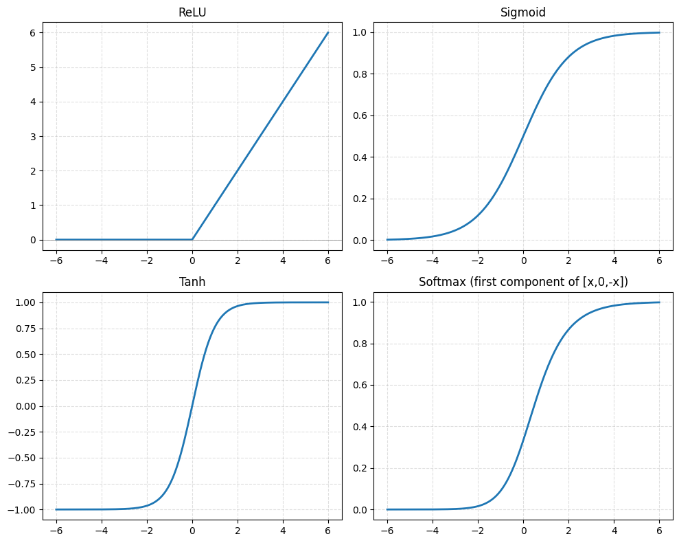
python
# inputs
x1 = Value(2.0, label='x1')
x2 = Value(0.0, label='x2')

# weights
w1 = Value(-3.0, label='w1')
w2 = Value(1.0, label='w2')

# bias of the nueuron
b = Value(6.8123512916312312331, label='b')

# x1*w1 + x2*w2 + b
x1w1 = x1*w1; x1w1.label = 'x1*w1'
x2w2 = x2*w2; x2w2.label = 'x2*w2'
x1w1x2w2 = x1w1 + x2w2; x1w1x2w2.label = 'x1*w1 + x2*w2'
n = x1w1x2w2 + b; n.label = 'n'
o = n.tanh(); o.label = 'o'

# 添加上 pow 和 div 运算
e = (2*n).exp()
o = (e - 1) / (e + 1); o.label = 'o'
o.backward()
python
draw_dot(o)
推导并计算神经网络的梯度
计算 do/dn
=> do/dn 套用公式得出 1 - tanh(n)**2
python
# 反向传播:1. 手动计算
# o.grad = 1
# n.grad = (1 - o.data**2) * o.grad

# b.grad = n.grad
# x1w1x2w2.grad = n.grad

# x1w1.grad = n.grad
# x2w2.grad = n.grad

# w1.grad = x1w1.grad * x1.data
# x1.grad = x1w1.grad * w1.data

# w2.grad = x2w2.grad * x2.data
# x2.grad = x2w2.grad * w2.data


# 反向传播:2. 半自动
# o.grad = 1
# o._backward()
# n._backward()
# x1w1x2w2._backward()
# x1w1._backward()
# x2w2._backward()


# 反向传播:3. 全自动
o.backward()
python
draw_dot(o)
正确计算梯度的“累加”效果
当一个变量被多次使用时,梯度是不是能正确地加起来
python
a = Value(3.0, label='a')
b = a + a; b.label = 'b'
b.backward()
python
draw_dot(b)
实现多层感知机 MLP
python
import random
class Module:
def zero_grad(self):
for p in self.parameters():
p.grad = 0
def parameters(self):
return []
class Neuron(Module):
def __init__(self, nin, nonlin=True):
self.w = [Value(random.uniform(-1,1)) for _ in range(nin)]
self.b = Value(0)
self.nonlin = nonlin
def __call__(self, x):
act = sum((wi*xi for wi,xi in zip(self.w, x)), self.b)
return act.relu() if self.nonlin else act
def parameters(self):
return self.w + [self.b]
def __repr__(self):
return f"{'ReLU' if self.nonlin else 'Linear'}Neuron({len(self.w)})"
class Layer(Module):
def __init__(self, nin, nout, **kwargs):
self.neurons = [Neuron(nin, **kwargs) for _ in range(nout)]
def __call__(self, x):
out = [n(x) for n in self.neurons]
return out[0] if len(out) == 1 else out
def parameters(self):
return [p for n in self.neurons for p in n.parameters()]
def __repr__(self):
return f"Layer of [{', '.join(str(n) for n in self.neurons)}]"
class MLP(Module):
def __init__(self, nin, nouts):
sz = [nin] + nouts
self.layers = [Layer(sz[i], sz[i+1], nonlin=i!=len(nouts)-1) for i in range(len(nouts))]
def __call__(self, x):
for layer in self.layers:
x = layer(x)
return x
def parameters(self):
return [p for layer in self.layers for p in layer.parameters()]
def __repr__(self):
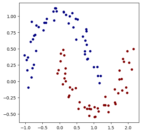
return f"MLP of [{', '.join(str(layer) for layer in self.layers)}]"案例:二元分类
python
import random
import numpy as np
import matplotlib.pyplot as plt
%matplotlib inline
python
np.random.seed(1337)
random.seed(1337)
python
from sklearn.datasets import make_moons, make_blobs
X, y = make_moons(n_samples=100, noise=0.1)

y = y*2 - 1 # make y be -1 or 1
# visualize in 2D
plt.figure(figsize=(5,5))
plt.scatter(X[:,0], X[:,1], c=y, s=20, cmap='jet')
<matplotlib.collections.PathCollection at 0x7bd161711100>
初始化一个 2 层神经网络模型
python
model = MLP(2, [16, 16, 1])
print(model)
print("number of parameters", len(model.parameters()))
MLP of [Layer of [ReLUNeuron(2), ReLUNeuron(2), ReLUNeuron(2), ReLUNeuron(2), ReLUNeuron(2), ReLUNeuron(2), ReLUNeuron(2), ReLUNeuron(2), ReLUNeuron(2), ReLUNeuron(2), ReLUNeuron(2), ReLUNeuron(2), ReLUNeuron(2), ReLUNeuron(2), ReLUNeuron(2), ReLUNeuron(2)], Layer of [ReLUNeuron(16), ReLUNeuron(16), ReLUNeuron(16), ReLUNeuron(16), ReLUNeuron(16), ReLUNeuron(16), ReLUNeuron(16), ReLUNeuron(16), ReLUNeuron(16), ReLUNeuron(16), ReLUNeuron(16), ReLUNeuron(16), ReLUNeuron(16), ReLUNeuron(16), ReLUNeuron(16), ReLUNeuron(16)], Layer of [LinearNeuron(16)]]
number of parameters 337
训练循环
python
epochs = 100
batch_size = 32

train_losses = []
train_accuracies = []

for epoch in range(epochs):

    # batch
    ri = np.random.permutation(X.shape[0])[:batch_size]
    Xb, yb = X[ri], y[ri]
    inputs = [list(map(Value, xrow)) for xrow in Xb]

    # forward
    scores = list(map(model, inputs))

    # svm loss
    batch_losses = [(1 + -yi*scorei).relu() for yi, scorei in zip(yb, scores)]
    data_loss = sum(batch_losses) * (1.0 / len(batch_losses))
    reg_loss = 1e-4 * sum((p*p for p in model.parameters()))
    total_loss = data_loss + reg_loss

    # accuracy
    accuracy = [(yi > 0) == (scorei.data > 0) for yi, scorei in zip(yb, scores)]
    acc = sum(accuracy) / len(accuracy)

    # backward
    model.zero_grad()
    total_loss.backward()

    # update
    lr = 1.0 - 0.9*epoch/100
    for p in model.parameters():
        p.data -= lr * p.grad

    train_losses.append(total_loss.data)
    train_accuracies.append(acc)

    if epoch % 1 == 0:
        print(f"epoch: {epoch} loss {total_loss.data}, accuracy {acc*100}%")
epoch: 0 loss 0.9821687249505938, accuracy 43.75%
epoch: 1 loss 2.7068597122644027, accuracy 78.125%
epoch: 2 loss 0.9272475020633426, accuracy 68.75%
epoch: 3 loss 0.7718329770328084, accuracy 75.0%
epoch: 4 loss 0.6178320975161242, accuracy 78.125%
epoch: 5 loss 0.257547153037419, accuracy 90.625%
epoch: 6 loss 0.2655796243711043, accuracy 90.625%
epoch: 7 loss 0.2193853494467976, accuracy 93.75%
epoch: 8 loss 0.1247642774978671, accuracy 96.875%
epoch: 9 loss 0.2854607191113145, accuracy 87.5%
epoch: 10 loss 0.2758215997744724, accuracy 87.5%
epoch: 11 loss 0.13380572155929976, accuracy 96.875%
epoch: 12 loss 0.30742299403549145, accuracy 87.5%
epoch: 13 loss 0.21817644569365738, accuracy 93.75%
epoch: 14 loss 0.3740226531169448, accuracy 84.375%
epoch: 15 loss 0.21245540666230645, accuracy 93.75%
epoch: 16 loss 0.18910051302410252, accuracy 93.75%
epoch: 17 loss 0.1616457986888311, accuracy 93.75%
epoch: 18 loss 0.18654849298127374, accuracy 90.625%
epoch: 19 loss 0.2370826459989099, accuracy 87.5%
epoch: 20 loss 0.10924022351149476, accuracy 96.875%
epoch: 21 loss 0.07153966099456222, accuracy 100.0%
epoch: 22 loss 0.110918898924129, accuracy 96.875%
epoch: 23 loss 0.21689654190230562, accuracy 90.625%
epoch: 24 loss 0.09279375812813531, accuracy 96.875%
epoch: 25 loss 0.2906949990088637, accuracy 87.5%
epoch: 26 loss 0.1956757141288569, accuracy 93.75%
epoch: 27 loss 0.4258814783164814, accuracy 84.375%
epoch: 28 loss 0.2977049401930041, accuracy 87.5%
epoch: 29 loss 0.07093172455546565, accuracy 100.0%
epoch: 30 loss 0.11271053483339821, accuracy 96.875%
epoch: 31 loss 0.09433820688436892, accuracy 96.875%
epoch: 32 loss 0.1736852423587532, accuracy 93.75%
epoch: 33 loss 0.13574629858868675, accuracy 93.75%
epoch: 34 loss 0.1381973581901792, accuracy 93.75%
epoch: 35 loss 0.2555137742865396, accuracy 90.625%
epoch: 36 loss 0.16332392924599196, accuracy 93.75%
epoch: 37 loss 0.2650792845492054, accuracy 90.625%
epoch: 38 loss 0.5108123607563144, accuracy 84.375%
epoch: 39 loss 0.28047553612647524, accuracy 87.5%
epoch: 40 loss 0.3237321790886433, accuracy 87.5%
epoch: 41 loss 0.19138261535130913, accuracy 93.75%
epoch: 42 loss 0.19893234843410956, accuracy 90.625%
epoch: 43 loss 0.06745377249411866, accuracy 100.0%
epoch: 44 loss 0.13647332951082336, accuracy 96.875%
epoch: 45 loss 0.09231527457440204, accuracy 96.875%
epoch: 46 loss 0.08856291401622467, accuracy 96.875%
epoch: 47 loss 0.01330432835412248, accuracy 100.0%
epoch: 48 loss 0.16481575083399094, accuracy 93.75%
epoch: 49 loss 0.09668757327007431, accuracy 96.875%
epoch: 50 loss 0.08052613843848216, accuracy 96.875%
epoch: 51 loss 0.1290206397858918, accuracy 93.75%
epoch: 52 loss 0.07094508408542559, accuracy 100.0%
epoch: 53 loss 0.19673713074055013, accuracy 93.75%
epoch: 54 loss 0.13268096485991823, accuracy 93.75%
epoch: 55 loss 0.0982770295051383, accuracy 93.75%
epoch: 56 loss 0.18597869385927557, accuracy 93.75%
epoch: 57 loss 0.08988561914809505, accuracy 96.875%
epoch: 58 loss 0.06508913873946214, accuracy 96.875%
epoch: 59 loss 0.04600696571140001, accuracy 100.0%
epoch: 60 loss 0.028805711916929058, accuracy 100.0%
epoch: 61 loss 0.150260119629409, accuracy 93.75%
epoch: 62 loss 0.05190158270318898, accuracy 96.875%
epoch: 63 loss 0.05168813153670566, accuracy 100.0%
epoch: 64 loss 0.09529271353299079, accuracy 96.875%
epoch: 65 loss 0.06504666227025055, accuracy 96.875%
epoch: 66 loss 0.07082564592401144, accuracy 100.0%
epoch: 67 loss 0.09899205684966106, accuracy 96.875%
epoch: 68 loss 0.061991489600069026, accuracy 96.875%
epoch: 69 loss 0.011013667722849804, accuracy 100.0%
epoch: 70 loss 0.026444791474337336, accuracy 100.0%
epoch: 71 loss 0.04175263021008844, accuracy 100.0%
epoch: 72 loss 0.10432026763271685, accuracy 96.875%
epoch: 73 loss 0.06752207931657601, accuracy 100.0%
epoch: 74 loss 0.13299609118323297, accuracy 96.875%
epoch: 75 loss 0.09873275152750062, accuracy 96.875%
epoch: 76 loss 0.03240352915767079, accuracy 100.0%
epoch: 77 loss 0.031177664917947344, accuracy 100.0%
epoch: 78 loss 0.10068018273483438, accuracy 93.75%
epoch: 79 loss 0.02912956944252348, accuracy 100.0%
epoch: 80 loss 0.04562880425398444, accuracy 96.875%
epoch: 81 loss 0.011075853877632038, accuracy 100.0%
epoch: 82 loss 0.061324032743785804, accuracy 96.875%
epoch: 83 loss 0.03968906929156545, accuracy 100.0%
epoch: 84 loss 0.04770400999847418, accuracy 96.875%
epoch: 85 loss 0.03119058662364043, accuracy 100.0%
epoch: 86 loss 0.018068092601941983, accuracy 100.0%
epoch: 87 loss 0.03425201370524789, accuracy 100.0%
epoch: 88 loss 0.022877059190229795, accuracy 100.0%
epoch: 89 loss 0.011096291699139378, accuracy 100.0%
epoch: 90 loss 0.07359267175676709, accuracy 96.875%
epoch: 91 loss 0.04793557692937296, accuracy 100.0%
epoch: 92 loss 0.017623415538430796, accuracy 100.0%
epoch: 93 loss 0.012154057050471342, accuracy 100.0%
epoch: 94 loss 0.011114585659607497, accuracy 100.0%
epoch: 95 loss 0.027735960523971263, accuracy 100.0%
epoch: 96 loss 0.014625945755114316, accuracy 100.0%
epoch: 97 loss 0.03195448441276933, accuracy 100.0%
epoch: 98 loss 0.03711281777474568, accuracy 100.0%
epoch: 99 loss 0.011121669097038586, accuracy 100.0%
绘制 loss 和 accuracy 曲线
python
import matplotlib.pyplot as plt

plt.figure(figsize=(10,4))

plt.subplot(1,2,1)
plt.plot(train_losses, label='Loss')
plt.xlabel('Step')
plt.ylabel('Loss')
plt.title('Training Loss')
plt.grid(True)
plt.legend()

plt.subplot(1,2,2)
plt.plot([a*100 for a in train_accuracies], label='Accuracy')
plt.xlabel('Epoch')
plt.ylabel('Accuracy (%)')
plt.title('Training Accuracy')
plt.grid(True)
plt.legend()

plt.tight_layout()
plt.show()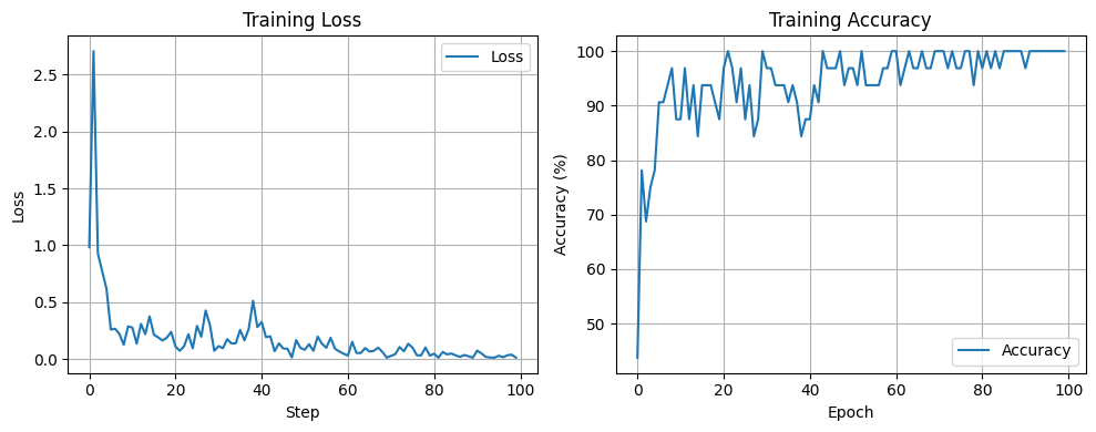
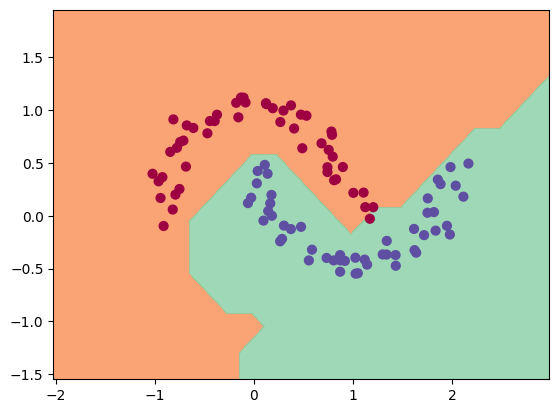
python
h = 0.25
x_min, x_max = X[:, 0].min() - 1, X[:, 0].max() + 1
y_min, y_max = X[:, 1].min() - 1, X[:, 1].max() + 1
xx, yy = np.meshgrid(np.arange(x_min, x_max, h),
                     np.arange(y_min, y_max, h))
Xmesh = np.c_[xx.ravel(), yy.ravel()]
inputs = [list(map(Value, xrow)) for xrow in Xmesh]
scores = list(map(model, inputs))
Z = np.array([s.data > 0 for s in scores])
Z = Z.reshape(xx.shape)

fig = plt.figure()
plt.contourf(xx, yy, Z, cmap=plt.cm.Spectral, alpha=0.8)
plt.scatter(X[:, 0], X[:, 1], c=y, s=40, cmap=plt.cm.Spectral)
plt.xlim(xx.min(), xx.max())
plt.ylim(yy.min(), yy.max())
(-1.548639298268643, 1.951360701731357)
总结
- 导数让我们理解单点变化率
- 偏导让我们知道多变量中每个方向的影响
- 梯度让我们找到下降最快的路径
- 链式法则让误差能顺利反传
- 梯度下降让模型学会自动优化
微积分让我们量化“变化”,链式法则让我们追踪“因果”,而梯度下降让机器能“学会”如何自己变得更好